Below is the living documentation of the Total Points system, which is Sports Info Solutions’ player value metric for football (NFL and CFB).
As updates get added to the system, we’ll add notes in this font to illustrate the most recent enhancements.
The most recent set of enhancements were made in August 2024.
What does Total Points do?
Total Points takes nearly everything that SIS measures about a play and uses it to evaluate each player on a scale that allows you to compare them more easily.
It’s always useful to be able to understand the different ways in which players can be valuable. Does he break a lot of tackles? Does he get a lot of yards after the catch? Does he make the best out of a poor offensive line? Total Points offers the opportunity to take all of those elements and get a quick picture of how well a player is performing overall.
What does the number mean?
All of Total Points uses the Expected Points Added (EPA) framework. EPA works by taking any given situation and finding the odds that each different scoring possibility comes next. For example, if the next scoring play is a field goal by the current defensive team two drives from now, you count that as a -3. Average those values across all instances of the same situation and you get its Expected Points. Take the change in Expected Points on any given play and you get its EPA.
Roughly, you can think of a 0 EPA play as one that “stays on schedule”, an EPA of 1 or more as a big play for the offense, and an EPA of negative-1 or less as a big play for the defense.
Total Points starts by evaluating each player on that scale, where 0 is average. That’s what we call Points Above Average. Then to both reward players who play full seasons and keep the sum of Total Points around what we’d expect a team to score or allow, we scale the results to the league scoring average (around 22 points per game). So when you see Josh Allen’s 171 leading quarterbacks in 2023, you could take that as a rough estimate that he contributed just about 10 points per game to the Bills’ scoring average on his own.
On the defensive side, it’s a little bit harder to wrap your mind around, because the scaling is exactly the same but points are bad for the defense. T.J. Watt’s 72 Points Saved in 2023 suggests that he was responsible for reducing his opponents’ scoring by that many points over the season.
How does it work?
We won’t go into complete detail here, but let’s run down the different data elements we consider, how they are evaluated in terms of EPA, and how they get bundled together.
Total Points works on each of the passing game and running game as a whole, so we’ll walk through them that way.
Pass Plays
Blocking
Everything starts up front. We start with identifying who was rushing the passer and who was blocking.
Then, those players are assigned a base value based on the expected value of the play overall. Starting in 2019, this takes into account drop type. Prior to 2019, this just involved whether the play was a screen pass.
Next, the line’s value is modulated by how long the play took to develop (starting in 2022). This uses our Expected Snap to Throw metric, and applies a multiplier to the baseline value corresponding to how much the timing of the play typically affects blown block rates (longer blocking, more credit for the line).
Then, we estimate how likely each person was to either blow a block (offense) or force a blown block (defense). On each play, credit is assigned to each player based on how they performed compared to that expectation, and the resulting blown block plus-minus value is multiplied by the average EPA of a blown block.
Players are additionally credited or debited if they were involved for good or for bad in a batted pass, deflection, or pressure, based on the average EPA of those events. For the 2019 season and beyond, our Pressures Above Expectation metric modulates the value assigned, with the form ({Pressure, No Pressure} – {Expected Pressure Rate}) x {Value of a Pressure}.
Pass Attempts
Each pass attempt gets split into five portions: throw, accuracy, catch, yards after catch before contact, and yards after contact.
- Throw: We take the value of the route at the intended depth in terms of its completion rate and interception rate. Starting in 2023, throw openness (contested, wide open, or in-the-middle) is incorporated as well.
- 75% owned by the quarterback, 25% owned by the receiver
- Accuracy: Comparing actual throw accuracy to expected accuracy, and multiplying the difference by the value of an accurate throw (based on expected catch and YAC rates). Starting in 2020, this uses our Expected On-Target Rate metric. Prior to 2020, it uses catchable throw rate, because we didn’t have enough granular accuracy data.
- 90% owned by the quarterback, 10% owned by the receiver
- Catch: Comparing actual completion success to expected catch rate, and multiplying the difference by the value of a completion (with expected YAC). Drops are considered completions for the passer. Uncatchable passes are not evaluated for the receiver.
- 10% owned by the quarterback, 90% owned by the receiver
- From 2020-22, this is 30/70 because we don’t have throw openness data. Prior to 2020, this is 50/50 because we don’t have granular accuracy data.
- Yards After Catch: Expected YAC is based on route, throw depth, and alignment. Starting in 2020, this includes granular throw accuracy. Starting in 2023, this includes throw openness. We give the receiver credit based on the difference in EPA between what he achieved and what was expected.
- 0% owned by the quarterback, 100% owned by the receiver
- From 2020-22, this is 40/60 because we don’t have throw openness data (and openness is the biggest driver of YAC). Prior to 2020, this is 50/50 because we don’t have granular accuracy data.
- Yards After Contact: Expected YACon is based on route, throw depth, and alignment. Starting in 2020, this includes granular throw accuracy. Starting in 2023, this includes throw openness. We give the receiver credit based on the difference in EPA between what he achieved and what was expected.
- 0% owned by the quarterback, 100% owned by the receiver
The defense at large takes responsibility for the throw itself because many factors contribute to the throw that’s selected, but the primary defender in coverage is responsible for the catch and yards after catch.
Any broken or missed tackles are evaluated according to their average EPA impact.
If the pass is intercepted, the quarterback and defender are equally debited and credited based on where the ball was caught. The defender then gets extra credit for the change in field position from his return.
All players running routes or defending in coverage have an expected target rate based on the coverage scheme, number of routes being run, route type, and alignment. Each player is assigned a value according to how many targets above expectation they had, scaled according to the EPA value of the potential target.
Pressure, Sacks, and Fumbles
Quarterbacks are given full responsibility for the sacks they incur (less the value of any blown blocks by the offensive line). They are given neither credit nor blame for pressure unrelated to blown blocks, with the idea that their throws are made more difficult but they also had some part in the pressure in the first place.
Sacks or evaded sacks are measured using the EPA of the sack (or potential sack) and an expected sack rate. The sacker(s) get full credit, unless it was deemed a coverage sack, in which case the coverage unit splits the credit. Starting in 2019, expected sack rate uses the Pressures Above Expectation framework.
Pass rushers are given credit for how well they generate pressures relative to the average of players lined up at the same position, with Pressures Above Expectation used from 2019 forward. Any pressure-related events that might have been debited from the line are given back to the receivers (and quarterback in the case of blown blocks), owing to their having a harder job as a result of the pressure.
All fumbles, recovered or lost, are evaluated similarly. The value of the potential turnover from that spot on the field is multiplied by the odds that possession will be lost based on whether it was in the backfield or not. Lamar Jackson was docked a lot of value for his 15 fumbles in 2018, even if the Ravens recovered most of them.
The person who recovers the fumble gets the inverse of the value that would be lost if the offense recovers or the “rest” of the fumble value if the defense recovers (i.e. the value of the turnover multiplied by the odds that it is recovered).
Pass Plays / Run Plays / Additional Adjustments / How to Use It
Run Plays
Blocking
Like with passing, the first step is to identify the blockers and box defenders. In addition, we use the intended and eventual run direction to identify the key blockers and defenders on the play (based on data elements like defensive techniques).
From there, we calculate the play’s expected yards before and after contact based on the number of box defenders, the blocking scheme, the run direction, the spot on the field, etc. The blockers are evaluated based on the play’s performance above that expectation, with most of the credit or blame going to the key blockers identified earlier (unless the runner cut the run back or bounced outside, in which case things are more balanced among blockers).
Starting in 2018, missed tackles (i.e. eluded without meaningful contact) that occur in the backfield are considered to be the point of contact for the purpose of evaluating the line.
The earlier the back is contacted on the play, the more responsibility the offensive line takes for the result of the play. That ranges from taking on 90% of the responsibility for plays that are blown up to 25% of the yards before contact beyond the first fifteen.
The same value is distributed among the box defenders, again focusing on the defenders at the intended gap. Blown blocks are evaluated similarly to what’s done in the passing game.
On plays where the back bounces or cuts the run back, the linemen initially run behind are evaluated differently from those who the back eventually runs behind. The extent of the difference depends on the direction and magnitude of the back’s movement. For example, cutbacks of 3 or more gaps are the most valuable bounce or cutback, so the value lost by the initial linemen is small because the cost of the cutback is small.
Rushing
The runner is evaluated against the offensive line’s expected performance calculated above. The rusher is given some credit for yards before contact because elusive runners can generate their own space, but most of his value will come after contact. The back’s responsibility for yards before contact increases the more yards he gains before contact, as it’s more likely he had a role in that result.
On any play where a broken or missed tackle was charted, we give the back a standard EPA amount based on the average value of a broken or missed tackle, with an adjustment for how likely an eluded tackle is on average. The EPA value is determined by comparing what happens when a tackle is made or eluded at the same yards downfield.
Fumbles are treated like they are on pass plays.
Tackling
Given each defender’s initial alignment, the heaviness of the box, and the run direction, we estimate the probability that each player would make the tackle and the EPA that would be expected if each of the possible defenders made the tackle.
A plus-minus system is used to combine the expected tackle rate and tackle value for each player and measure that against whether the player actually recorded a tackle. That system is also modified to ensure that making a tackle is always better than not making one, regardless of the value of said tackle compared to expectation.
Broken or missed tackles are taken independent of where they are on the field, so each one is considered worth the value of an average broken or missed tackle in terms of EPA.
Pass Plays / Run Plays / Additional Adjustments / How to Use It
Additional Adjustments
Play Selection
At this point it’s common knowledge that run plays are less valuable on average than pass plays. At a basic level we can see this because the average yards per attempt on passes is much higher than it is on runs. In a similar way, play action passing is generally more effective than straight dropback passing.
At a more granular level, coaches can make inefficient decisions by electing to, for example, run from heavy personnel on second-and-10.
In order to more accurately evaluate the players on a play as opposed to the coaches or situations, we implemented a Play Selection Adjustment, which applies to each player on each play. We take the expected value of the play given the run/pass decision—including whether there was a play fake on a dropback—and some personnel and game state information, compare it to an average play, take the difference, and distribute that value among the players involved. That way, a back being run into a heavy box time and again isn’t punished simply for being on the field in a sub-par situation for him.
This adjustment generally moves a player a handful of points one way or the other depending on how often he was involved in pass or run plays over the course of a season.
Season Scoring
As mentioned above, after all of the initial calculations are done, we re-scale everything so that the league total is in line with the league’s scoring average, or just over 22 points per team per game. Because the quarterback represents the most obviously critical position, he’s given 1/3 of this adjustment for the offense, and the rest is split among the other offensive players.
The Gist
Let’s say that you read all this stuff and already kind of forget what you read at the beginning. Here’s a quick-and-dirty version:
- We take Expected Points Added and give individual value to every player on every scrimmage play, starting in 2016
- You can find it on the SIS DataHub player pages and leaderboards. Here’s the leaderboards for quarterbacks, offensive linemen, defensive linemen, and defensive backs as examples. The SIS DataHub Pro offers more detailed filtering ability and even more in-depth stats.
- Pass Offense: Quarterbacks and receivers split value for the throw, the catch, after-catch yards, and after-contact yards. Additional considerations for offensive line performance, uncatchable passes, and drops.
- Pass Defense: Defensive backs are measured on how often they are targeted above expectation, and much of the value that the receivers or QB get on a completion is correspondingly taken away from the defender. Pass rushers are credited for forcing blown blocks and disruptions at the point of attack.
- Rush Offense: The offensive line and running back both take responsibility for yards before contact (weighted towards the O-line), while yards after contact beyond what’s expected are totally owned by the back. Broken tackles hold a lot of value.
- Rush Defense: Preventing yards before contact is the name of the game for the defensive line, while linebackers and defensive backs get value from making tackles that limit yardage compared to expectation and not missing out on easy tackle opportunities.
- In general, there’s a lot of value to be gained and lost from turnovers (or turnover-worthy plays) and plays in key spots (e.g. just outside field goal range, third down).
Pass Plays / Run Plays / Additional Adjustments / How to Use It
What do we do with it?
Now that you’re familiar with what goes into Total Points, what do you do with it?
The first thing you might do is find players whose traditional stats or reputation don’t line up with their rank in Total Points.
How was Lamar Jackson barely above zero value rushing in 2018? You saw the reason for that above (his propensity to fumble).
Why was James Conner such a standout in 2023, even above Offensive Player of the Year Christian McCaffrey? He had a worse offensive line and was elite when it came to yards after contact, production that he doesn’t split with anyone.
Total Points gives us the opportunity to more critically engage with the stats players compile and consider the context in which he compiled them. And as SIS continues to add more data points to its operation, our assessment of those things will only get better.


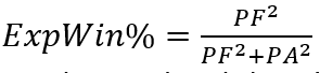 and use partial derivatives to convert it into a formula for points-per-win at a league level that depends only on the scoring environment (in points per game, PPG):
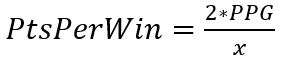 , where x is the
  value that makes the Pythagorean win expectancy most accurate when it’s used as the exponent instead of squaring each term. For 2016 to 2019, with a PPG just over 45, z = 0.73.